Getting Started
LOBSTER is an image analysis environment to identify biological objects in microscopy images, and measure their spatial location, geometry, dynamics and intensity distribution. The objects can be exported as 2D/3D models, for instance for their exploration/edition in external software, or for the simulation of the processes under study. Multiple images can be processed in one go and image size is not limited by the main memory of the workstation.
Setting Up
Assuming that MATLAB (version >=2015a), Image processing and Statistics & Machine Learning toolboxes are installed:
- Download the source code (green button)
- Unzip the content to an empty folder where MATLAB has write access
- Create an empty folder /Images inside the installation folder and unzip this archive (sample images)
- Create an empty folder /Results inside the installation folder and unzip this archive (sample results).
Initializing
Launch MATLAB and type the following lines from the console:
>> cd E:/LOBSTER (update path to installation folder)
>> init
LOBSTER Panel
To start the Panel, type >> LOBSTER.
From this interface, you can load up to 2 object identification workflows (journals), trigger object measurements and export object models. To load a journal, click Journal1 and select its file from the browser (for instance 'Tissue_SegWaterTiles.jl').
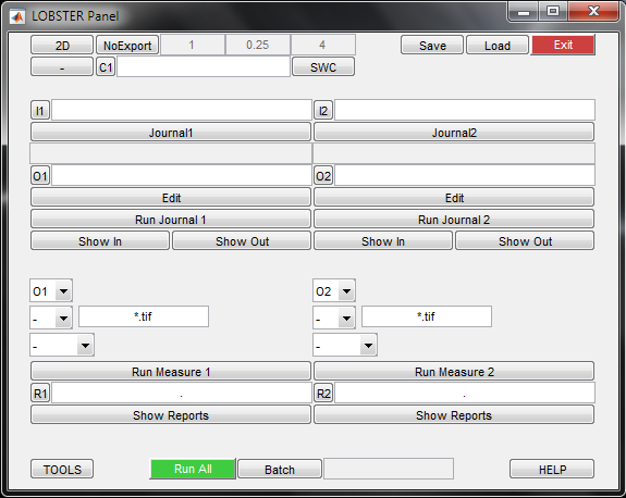
The input and output folders are parsed from the journal and displayed in the fields I and O. It is also possible to edit the path to these folders to use existing journals to process different images.
To launch the journal, click Run Journal 1. By default, no image is displayed (batch mode), this behaviour can be modified by pressing the Batch button located at the bottom of the panel. The images from the input folder are processed sequentially, and they are displayed together with the results from the workflow configured in the journal. Press 'm' to toggle the display of the results, and 'x' to proceed to the next image. To stop the processing when an image is displayed, press 'q'. To stop the processing while an operation is performed, press CTRL+C.
If the results are not satisfactory, tweak the journal parameters from the editor (Edit), save it (floppy disk) and launch it again. From the journal editor, press F1 while hovering over a function (@) to get help on its parameters. Once the results are satisfactory, set batch mode and launch the journal on all input images. The input and output folders of a journal can be browsed by clicking Show In and Show Out. This is illustrated in this video, in this case the journal is called from console, and the folders are browsed from console hyperlinks. To get more information on journals, refer to this page, but this is not strictly necessary at this point.
To perform measurements on the objects identified by Journal1, set the upper drop-down selector (object mask folder) to O1 (that is, the output of Journal 1) and set the lower drop-down selector to 'Objs' (plain objects measurements). Press Run Measure 1. Upon completion, press Show Reports to browse the folder holding the CSV reports.
Journal processing and measurements can be performed in one go by pressing Run All. The current operation is displayed in the bottom right field and Run all is set to red to show until all images are processed. Refer to the context help provided when hovering over the other items.
Sample Projects
Several sample projects are described in this section, the corresponding files (.mat) can be found in LOBSTER /Projects folder. It is possible to open an existing project by clicking Load.
Tracing blood vessels from 3D images
Tracing blood vessels from 3D images, exporting to SWC format and visualizing the 3D models.
Load project 'BloodVesselsTracing.mat', click Run All and visualize resulting .SWC files by loading them from this webpage.
Segmenting nuclei from 3D images
Segmenting nuclei from 3D images, exporting to STL format and visualizing the meshes.
Load project 'CellPilar3DMesh.mat', click Run All and visualize the STL meshes by drag and dropping them to this web page. For larger meshes, it is recommended to use MeshLab.
Exporting detected nuclei as an ImageJ interactive montage
Drag and drop the report file (.csv) from the previous project to ImageJ, open the input image and run the macro Tools/Montager.ijm. This builds an interactive montage of all detected objects: clicking an object in the montage jumps to its position in the original image. The input image can also be opened in virtual stack mode to handle large images not fitting in main memory (drag and drop the image to ImageJ bar >> symbol so that Open as Virtual Stack is displayed).Tracking dividing nuclei from a 2D time-lapse
Segmenting 2D objects from a time-lapse, tracking the objects, exploring results in ImageJ and plotting in Matlab.
Load project 'HeLaTracking.mat'. This project performs the segmentation and tracking of dividing nuclei from a sequence of 2D images. TL is enabled to specify that Journal2 is a time-lapse journal perfroming tracking (.jlm extension).
This time, I2 points to O1 since the images are first segmented into object masks (Journal 1) before being tracked (Journal 2).
When running the first journal, an image window pops up at the end of the processing. This is because the tracker (Journal 2) requires the best possible segmentation mask at first time point. To this end, the user needs to correct erroneous object splitting (most common errors) by drawing small rectangles around false cut lines (hold mouse left button). Beware to maximize the image window (or zoom around), to make sure that all objects are properly merged. Exit mask correction by clicking on the image.
Measuring O2 (Object masks) brings 3 report files: objects areas, CMx and CMy (objects centroids). Tracking results can be visualized from ImageJ macro Tools/OverlayTrackedObjects.ijm by selecting O1 as input folder and O2 as output folder.
To plot some of the measurements, type PlotTrksMeasurements in MATLAB and select the .csv file of the measurement you want to plot. Type the ID of the objects you want to plot.
Tracking nuclei from a 3D time-lapse
Segmenting 3D objects from a time-lapse, tracking the objects and exploring the tracks in Mastodon.
Load project 'Mastodon3D_Test.mat' and click Run All. To visualize the 3D tracks, an amazing tool is Mastodon, leveraging the awesome ImageJ Big Data Viewer. To use Mastodon, it is first required to convert the input image to Big Data Viewer format by opening the image in ImageJ and calling Plugins > BigDataViewer > Export Current Image as XML/HDF5. Before doing so, make sure the dimensions are right from Image>Properties (especially Z and T). It is recommended to export the image to the same folder as the input image folder and with the default name (export.xml).
LOBSTER tracks can be converted to a format importable by Mastodon by typing MamutExport in Matlab console, and selecting the required files/folders: the XML input file should be in Images/Mastodon3D/export.xml and tracking / report folders are respectively O2 and R2 for this project.
Upon conversion, open Mastodon from ImageJ. Click New project in Mastodon window and select the input image XML file (export.xml). Click import mamut and select export_mamut.xml. Click bdv and trackscheme access to the image and track viewers. It is possible to edit the tracks and perform other operations. Refer to Mastodon documentation for reference.
Note: If you want to try Mastodon with object divisions, export the time-lapse from the previous project as XML/HDF5 and perform the same operations.
Detecting nuclei from 3D images
Detecting nuclei from 3D images, exporting the markers to LOBSTER CellInsight and editing them.
Load project 'LymphGlandCellInsight.mat', click Run All. Open ImageJ and drag and drop the macro CellInsight (click TOOLS button to access tools folder).
Note: The first time you use CellInsight, it is required to copy the file GetString.ijm to ImageJ /macros folder.
Drag and drop the input image to ImageJ (click Show In to browse input folder). Launch CellInsight.ijm from ImageJ macro editor, and press Import to load LOBSTER object markers. The object markers can be explored and edited (see CellInsight documentation). Exit CellInsight by clicking Exit, not by closing the image in ImageJ.
Note: Large images not fitting in main memory can be opened in virtual stack mode (drag and drop the image to ImageJ bar >> until Open as Virtual Stack is displayed).
Counting FISH spots inside nuclei
Load the project 'FISH.mat'. This project holds two journals: the first journal identifies nuclei (DAPI channel) and the the second journal identifies FISH signals (seed mask, one non null pixel per spot). The aim is to count the number of FISH markers inside every nucleus. The source object mask for Measure 1 is set to O1 (nuclei mask, output of Journal 1) since we want to measure nuclei, and the drop-down selector right below (intensity measurement channel) is set to O2 (Journal2 output): this is because we want to count the number of FISH markers per nucleus (number of non null pixels in FISH seed mask). The general principles of how object masks are used to perform measurements is detailed in this section.Note: In this particular case, since both journals point to the same input folder, the channel selection (DAPI/FISH) is performed inside the journals. To understand how, you can refer to this page.
Processing large 3D images
To process large 3D images, bricking should be enabled by defining the variable Brick in the journal. For example, load the project 'CellPilar_brcks.mat' and inspect the journal (Edit): the variable Brick is set to 128 and the variable GaurdBand is set to 64. Both JENI and IRMA process the image by bricks of size 128 x 128, with an overlap of 64 pixels between bricks.
If needed, it is possible to convert bricked output masks to regular masks (folder of image slices) by typing ExportBricksAsSlices in MATLAB console. Select one of the folders (output image) from the output folder (here O1) and an empty folder to export the slices.
Architecture
Objects identification, measurements and modeling are performed sequentially and the results are stored in simple formats after each step. These operations are respectively performed by three computational modules called from MATLAB console (scripting) or LOBSTER Panel (Graphical User Interface). In this tutorial we cover the Panel, refer to this page for scripting.
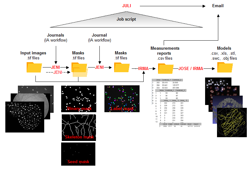
JENI: Identifying objects
All TIFF images from an input folder are typically processed into object masks by applying a sequence of image analysis functions (workflow) configured in a journal (short text file). The object masks can be of four kinds illustrated in the figure above:
- Binary masks ('Objs'): objects encoded as connected groups of foreground pixels
- Skeleton masks ('Skls'): 1-pixel curves marking filament centrelines
- Seed masks ('Spts'): foreground pixels mark objects
- Label masks ('Trks'): objects encoded as connected groups of pixels with same intensity level (unique ID).
IRMA: Measuring object masks
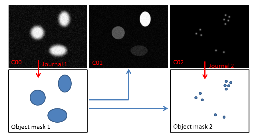
Object masks can be used to measure objects or become the basic building blocks of more complex workflows. For instance, in the figure above Object Mask 1 is both used to measure C01 intensity and count the number of C02 objects inside C00 objects. Objects masks can also be used for object based co-localization study, or to extract relative object distance distributions (e.g. spots to filaments). All object measurements are performed by IRMA from the object masks, and results are exported to .csv reports.
JOSE/IRMA: Exporting object models
Identified objects can be exported as 2D/3D models so as to be explored externally: filaments networks are exported as SWC or OBJ models, object surfaces are exported as STL meshes and object tracks are exported as SWC trees. Finally, object markers can be exported as CellInsight files (.xls), an ImageJ macro (provided in /Tools folder) enabling to edit and visualize them.
Using LOBSTER for your own Application
Designing practical journals and becoming familiar with LOBSTER functions can take some practice. To get started, the best approach is probably to test and adapt existing journals since many sample journals and companion images are provided (see LOBSTER documentation Appendix - Applications for the complete list). Here is how you can process:
- Look for a journal performing at least part of the analysis you plan
- Run the journal to see the input images and get a feeling about the results
- Make a copy of the journal and modify it to point to your input image folder (for large images, you probably first want to crop out some illustrative regions)
- Make sure that your images have the same bit depth than the images of the journal, if not convert them or adapt the parameters of the journal if needed
- Run the journal
- You will probably need to tweak the parameters of some of the functions to obtain satisfactory results.
- Completing the project might finally require some customization, such as combining multiple journals and performing cross-measurements or exporting object models (such as illustrated in the previous section).
Read On
Some more features are available in LOBSTER, refer to the complete documentation for more details. Also read on details about journals and scripting to build projects involving more that two journals or perform advanced operations.